How to get relative row numbers in a range in Excel

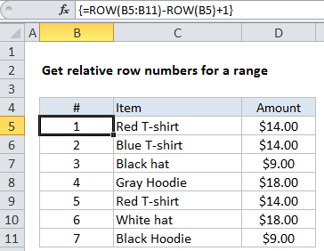
To get a full set of relative row numbers in a range, you can use an array formula based on the ROW function. See example below;

Formula

{=ROW(range)-ROW(range.firstcell)+1}

Note: this is an array formula that must be entered with Control + Shift + Enter. If you’re entering this on the worksheet (and not inside another formula), make a selection that includes more than one row, enter the formula, and confirm with Control + Shift + Enter.

Explanation

In the example shown, the formula in B5:B11 is:

{=ROW(B5:B11)-ROW(B5)+1}

This is formula will continue to generate relative numbers even when the range is moved. However, it’s not a good choice if rows need to be sorted, deleted, or added, because the array formula will prevent changes.

How this formula works

The first ROW function generates an array of 7 numbers like this:

{5;6;7;8;9;10;11}

The second ROW function generates an array with just one item like this:

{5}

which is then subtracted from the first array to yield:

{0;1;2;3;4;5;6}

Finally, 1 is added to get:

{1;2;3;4;5;6;7}

Generic version with named range

With a named range, you can create a more generic version of the formula using the MIN function or the INDEX function. For example, with the named range “list”, you can use MIN like this:

{ROW(list)-MIN(ROW(list))+1}

With INDEX, we fetch the first reference in the named range, and using ROW on that:

{=ROW(list)-ROW(INDEX(list,1,1))+1}

You’ll often see “relative row” formulas like this inside complex array formulas that need row numbers to calculate a result.