How to get address of last cell in range in Excel

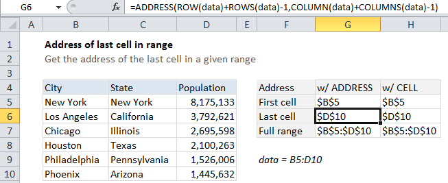
In the example shown, the formula in G6 is:

=ADDRESS(ROW(data)+ROWS(data)-1,COLUMN(data)+COLUMNS(data)-1)

How this formula works

The ADDRESS function builds an address based on a row and column number.

Working from the inside out, we use the ROW function to generate a list of row numbers, which are then shifted by adding ROWS(data)-1,  so that the first item in the array is the last row number:

ROW(data)+ROWS(data)-1

Then we do the same thing with COLUMN and COLUMNS:

COLUMN(data)+COLUMNS(data)-1

The ADDRESS function then assembles and returns an array of addresses. When entered in a single cell, just the item from the array is displayed, which is the address corresponding to the last cell in a range.

CELL function alternative

You can also use the CELL function to get the address of the last cell in a range with this formula:

=CELL("address",INDEX(data,ROWS(data),COLUMNS(data)))

In this case, we use INDEX to get a reference to the last cell in the range, which we determine by passing total rows and total columns into INDEX. The reference returned by INDEX is then handled by the CELL function, using “address”, to return the address.

Note that the the CELL function can be volatile. If you add it to a worksheet, you’ll notice that you are prompted to save even when you’ve made no changes.