Get nth match with INDEX / MATCH in Excel

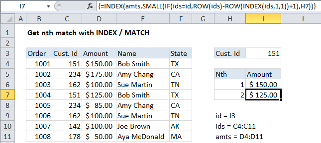
To retrieve multiple matching values from a set of data with a formula, you can use the IF and SMALL functions to figure out the row number of each match and feed that value back to INDEX. In the example shown, the formula in I7 is:

{=INDEX(amts,SMALL(IF(ids=id,ROW(ids)-ROW(INDEX(ids,1,1))+1),H6))}

Where named ranges are amts (D4:D11), id (I3), and ids (C4:C11).

Note that this is an array formula and must be entered with Control + Shift + Enter.

How this formula works

At the core, this formula is simply an INDEX formula that retrieves the value in an array at a given position. The value for n  is supplied in column H, and all the “heavy” work that the formula does is to figure out the row from which to retrieve a value, where row corresponds to “nth” match.

The IF function does the work of figuring out which rows contain a match, and the SMALL function returns the nth value from that list. Inside of IF, the logical test is:

ids=id

which yields this array:

{TRUE;FALSE;FALSE;TRUE;FALSE;FALSE;FALSE}

Note the customer id matches at the 1st and 4th positions, which appear as TRUE. The “value if true” argument in IF generates a list of relative row numbers with this expression:

ROW(ids)-ROW(INDEX(ids,1,1))+1

which produces this array:

{1;2;3;4;5;6;7}

This array is then “filtered” by the logical test results, and the IF function returns the following array result:

{1;FALSE;FALSE;4;FALSE;FALSE;FALSE}

Note we have valid row numbers for row 1 and row 2.

This array is then processed by SMALL, which is configured to use values in column H to return “nth” values. The SMALL function automatically ignores the logical values TRUE and FALSE in the array. In the end, the formulas reduce to:

=INDEX(amts,1) // I6, returns $150
=INDEX(amts,4) // I7, returns $125

Handling errors

Once there are no more matches for a given id, the SMALL function will return a #NUM error. You can handle this error with the IFERROR function, or by adding logic to count matches and abort processing once the number in column H is greater than the match count. The example here shows one approach.