Find closest match in Excel

This tutorial shows how to Find closest match in Excel using the example below;

Formula

{=INDEX(data,MATCH(MIN(ABS(data-value)),ABS(data-value),0))}

Explanation

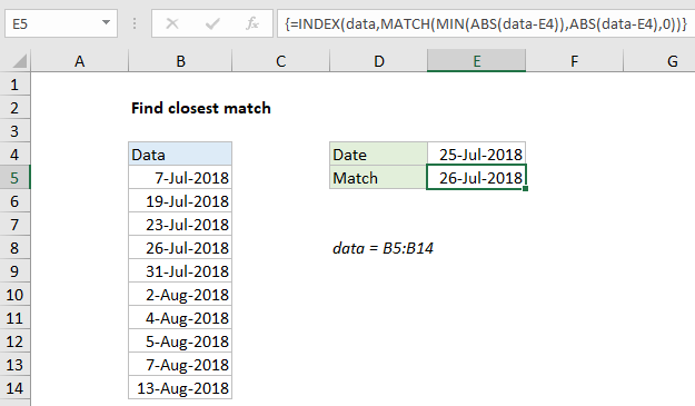
To find the closest match with a lookup value and numeric data, you can use an array formula based the INDEX, MATCH, ABS and MIN functions. In the example shown, the formula in E5 is:

{=INDEX(data,MATCH(MIN(ABS(data-E4)),ABS(data-E4),0))}

where “data” is the named range B5:B14, and E4 contains a lookup value.

Note: this is an array formula and must be entered with control + shift + enter.

How this formula works

At the core, this is an INDEX and MATCH formula where MATCH locates the position of the closest match and feeds that postion into INDEX. INDEX then returns the value at that position. All of the hard work is done inside the MATCH function, which is configured like this:

MATCH(MIN(ABS(data-E4)),ABS(data-E4),0)

Inside MATCH, this expression calculates the differences between the lookup value in E4 and the values in the named range data:

data-E4

This is an array expression, and it returns and array result like this:

{-18;-6;-2;1;6;8;10;11;13;19}

The ABS function is then used to convert negative values to positive:

{18;6;2;1;6;8;10;11;13;19}

These values represent the difference between the lookup value and the values in data. We are looking for the closest match,  so we use the MIN function to return the smallest value. In this case, the smallest value is 1, and this becomes the lookup value inside MATCH.

The lookup array is calculated in a similar way. The expression:

ABS(data-E4)

returns the following array to MATCH as the lookup array:

{18;6;2;1;6;8;10;11;13;19}

The last argument inside MATCH is match_type, which is set to zero to force an exact match.

Finally, with these values, the MATCH function returns the position of 1 inside the array, which is 4. The position is fed into INDEX as the row argument:

=INDEX(data,4)

The INDEX function then returns the value at that position, which is the date July 26, 2018.

Note: in the event of a tie, this formula will return the first match.

Click link for more examples on how to find closest match in Excel.