Approximate match with multiple criteria in Excel

To lookup and approximate match based on more than one criteria, you can use an array formula based on INDEX and MATCH, with help from the IF function.

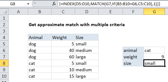
In the example shown, the formula in G8 is:

{=INDEX(D5:D10,MATCH(G7,IF(B5:B10=G6,C5:C10),1))}

Note: this is an array formula and must be entered with Control + Shift + Enter

The goal of this formula is to return “size” when given an animal and a weight.

How this formula works

At the core, this is just an INDEX / MATCH formula. The problem in this case is that we need to “screen out” the extraneous entries in the table so we are left only with entries that correspond to the animal we are looking up.

This is done with a simple IF function here:

IF(B5:B10=G6,C5:C10)

This snippet tests the values in B5:B10 to see if they match the value in G6 (the animal). Where there is a match, the corresponding values in C5:C11 are returned. Where there is no match FALSE is returned. When G6 contains “cat”, the resulting array looks like this:

{FALSE;FALSE;FALSE;5;10;15}

This goes into the MATCH function as the array. The lookup value for match comes from G7, which contains the weight (9 lbs in the example).

Note that match is configured for approximate match by setting match_type to 1, and this requires that the values in C5:C11 must be sorted.

MATCH returns the position of the weight in the array, and this is passed to INDEX as the row number. The lookup_array for INDEX are the sizes in D5:D10, so INDEX returns a size corresponding to the position generated by MATCH (the number 4 in the example shown).