
Skip to content
Free Excel Tutorials
  • Home
  • Excel For Beginners
  • Excel Intermediate
  • Advanced Excel For Experts

Data Analysis

  • Reverse List in Excel
  • How To Compare Two Lists in Excel
  • How to combine 2 or more chart types in a single chart in Excel
  • How to add Trendline to a chart in Excel
  • How To Create Pareto Chart in Excel

References

  • How to get relative column numbers in a range in Excel
  • VLOOKUP function: Description, Usage, Syntax, Examples and Explanation
  • Find closest match in Excel
  • How to reference named range different sheet in Excel
  • Lookup entire row in Excel

Data Validations

  • Excel Data validation don’t exceed total
  • Excel Data validation date in specific year
  • Excel Data validation specific characters only
  • Excel Data validation unique values only
  • Data validation must not exist in list

Example of payment for annuity in Excel

by

This tutorial shows how to solve for an annuity payment in Excel. An annuity is a series of equal cash flows, spaced equally in time.

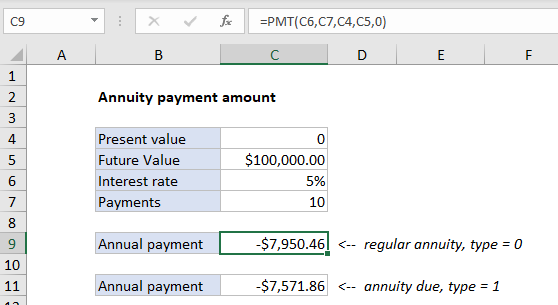
Case study:  Using the PMT function, the goal in this example is to have 100,000 at the end of 10 years, with an interest rate of 5%. Payments are made annually, at the end of each year.

Formula

=PMT(rate,nper,pv,fv,type)
Explanation

In the example shown C9 contains this formula:

=PMT(C6,C7,C4,C5,0)

Explanation

To solve for the payment required, the PMT function is configured like this:

  • nper – from cell C7, 25.
  • pv – from cell C4, 0.
  • rate – from cell C6, 5%.
  • fv – from cell C5, 100000.
  • type – 0, payment at end of period (regular annuity).

With this information, the PMT function returns -$7,950.46. The value is negative because it represents a cash outflow.

Annuity due

With an annuity due, payments are made at the beginning of the period, instead of the end. To calculate the payment for an annuity due, use 1 for the type argument. In the example shown, the formula in C11 is:

=PMT(C6,C7,C4,C5,1)

which returns -$7,571.86 as the payment amount. Notice the only difference in this formula is type = 1.

Post navigation

Previous Post:

DECIMAL function: Description, Usage, Syntax, Examples and Explanation

Next Post:

AVERAGE function: Description, Usage, Syntax, Examples and Explanation

Leave a Reply Cancel reply

Your email address will not be published. Required fields are marked *

Learn Basic Excel

Ribbon
Workbook
Worksheets
Format Cells
Find & Select
Sort & Filter
Templates
Print
Share
Protect
Keyboard Shortcuts

Categories

  • Charts
  • Data Analysis
  • Data Validation
  • Excel Functions
    • Cube Functions
    • Database Functions
    • Date and Time Functions
    • Engineering Functions
    • Financial Functions
    • Information Functions
    • Logical Functions
    • Lookup and Reference Functions
    • Math and Trig Functions
    • Statistical Functions
    • Text Functions
    • Web Functions
  • Excel VBA
  • Excel Video Tutorials
  • Formatting
  • Grouping
  • Others

Logical Functions

  • IF with wildcards in Excel
  • Check multiple cells are equal in Excel
  • IFERROR function: Description, Usage, Syntax, Examples and Explanation
  • How to use Excel AND Function
  • Invoice status with nested if in Excel

Date Time

  • HOUR function: Description, Usage, Syntax, Examples and Explanation
  • Get month name from date in Excel
  • Two ways to sum time over 30 minutes in Excel
  • Convert decimal minutes to Excel time
  • Add decimal minutes to time in Excel

Grouping

  • If cell contains one of many things in Excel
  • Map text to numbers in Excel
  • How to randomly assign people to groups in Excel
  • How to randomly assign data to groups in Excel
  • Group numbers at uneven intervals in Excel

General

  • How to test a range for numbers in Excel
  • How to increase by percentage in Excel
  • Cell References: Relative, Absolute and Mixed Referencing Examples
  • Excel Autofill Cell Ranges, Copy, Paste
  • Subtotal by color in Excel
© 2026 xlsoffice . All Right Reserved. | Teal Smiles | Abbreviations And Their Meaning