Get days, hours, and minutes between dates in Excel

To calculate and display the days, hours, and minutes between two dates, you can use the TEXT function with a little help from the INT function. Alternatively, you can adapt the formula using SUMPRODUCT.

Formula

=INT(end-start)&" days "&TEXT(end-start,"h"" hrs ""m"" mins """)

Explanation

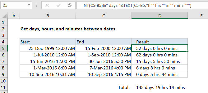
In the example shown, the formula in D5 is:

=INT(C5-B5)&" days "&TEXT(C5-B5,"h"" hrs ""m"" mins """)

How this formula works

Most of the work in this formula is done by the TEXT function, which applies a custom number format for hours and minutes to a value created by subtracting the start date from the end date.

TEXT(C5-B5,"h"" hrs ""m"" mins """)

This is an example of embedding text into a custom number format, and this text must be surrounded by an extra pair of double quotes.

The value for days is calculated with the INT function, which simply strips off the integer portion of the end date minus the start date:

INT(C5-B5)

Although you can use “d” in a custom number format for days, the value will “roll over” back to zero when days is greater than 31.

Include seconds

To include seconds, you can extend the custom number format like this:

=INT(C5-B5)&" days "&TEXT(C5-B5,"h"" hrs ""m"" mins ""s"" secs""")

Total days, hours, and minutes between dates

To get the total days, hours, and minutes between a set of start and end dates, you can adapt the formula using SUMPRODUCT like this:

=INT(SUMPRODUCT(ends-starts))&" days "&TEXT(SUMPRODUCT(ends-starts),"h"" hrs ""m"" mins """)

where “ends” represents the range of end dates, and “starts” represents the range of start dates. In the example shown, D11 contains this formula:

=INT(SUMPRODUCT(C5:C9-B5:B9))&" days "&TEXT(SUMPRODUCT(C5:C9-B5:B9),"h"" hrs ""m"" mins """)