Dynamic date list in Excel

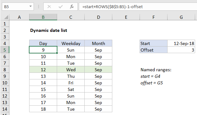
This tutorial show how to Dynamic date list in Excel using the example below.

To create a dynamic date list, you can use a formula that increments a start date to create and display additional dates.

 Formula

=start+ROWS(exp_rng)-1-offset

Explanation of how this formula works

In the example shown, the formula in B5 is:

=start+ROWS($B$5:B5)-1-offset

where “start” is the named range G4, and “offset” is the named range G5.

Notes: (1) the offset represents days before the start date to display in the list. (2) the shading of the start date is done with conditional formatting as described below.

Dates in Excel are just serial numbers, formatted to display as dates. This means you can perform math operations on dates to calculate days in the future or past.

In the example shown, the date in the named range “start” is provided by the TODAY function:

=TODAY() //returns current date

The formula in B5 begins with the start date, and increments the date by one using an expanding range inside the ROWS function:

ROWS($B$5:B5) // returns row count

ROWS returns the row count in a range. As the formula is copied down, the range expands and the row count increases by one at each new row. From this value, we subtract 1, so the date is not incremented in the first row.

Next, we subtract the value in in the named range “offset” (G5). The offset is simply a way to begin the list of dates earlier than the start date provided. If offset is zero or blank, the first date in the list will equal the start date.

To display a month, the formula in D5 is:

=TEXT(B5,"mmm")

To display a weekday, the formula in C5 is:

=TEXT(B5,"ddd")

The formulas in B5, C5, and D5 can be copied down as many rows as desired.

Highlighting the start date

The start date is shaded with a conditional formatting rule based on this formula:

=$B5=start