How to conditionally sum numeric data in an Excel table using SUMIFS

To conditional sum numeric data in an Excel table, you can use SUMIFS with structured references to for both sum and criteria ranges.

Formula

=SUMIFS(Table[sum_col],Table[crit_col],criteria)

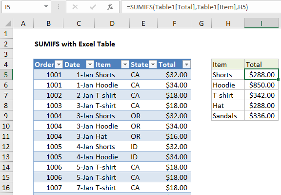
In the example shown, the formula in I5 is:

=SUMIFS(Table1[Total],Table1[Item],H5)

Where Table1 is an Excel Table with the data range B105:F89.

This formula uses structured references to feed table ranges into the SUMIFS function.

The sum range is provided as Table1[Total], the criteria range is provided as Table1[Item], and criteria comes from values in column I.

The formula in I5 appears like this:

=SUMIFS(Table1[Total],Table1[Item],H5)

And resolves to this:

=SUMIFS(F5:F89,D5:D89,"Shorts")

The SUMIFS function returns 288, the sum values in the Total column where the value in the Item column is “Shorts”.