Conditional Formatting New Rule with Formulas in Excel

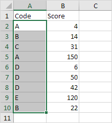
If the Highlight Cells Rules, Top/Bottom Rules, Data Bars, Color Scales and Icon Sets are not sufficient, you can create a new rule. For example, highlight the codes below that occur more than once in the range A2:A10 andhave a score greater than 100.

1. Select the range A2:A10.

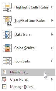
2. On the Home tab, in the Styles group, click Conditional Formatting.

3. Click New Rule.

Note: Highlight Cells Rules, Top/Bottom Rules, Data Bars, Color Scales and Icon Sets are shortcuts. They can also be found under New Rule.

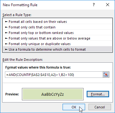
4. Select ‘Use a formula to determine which cells to format’.

5. Enter the formula =AND(COUNTIF($A$2:$A$10,A2)>1,B2>100)

6. Select a formatting style and click OK.

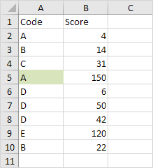
Result. Excel formats cell A5 because code A occurs more than once in the range A2:A10 and the value 150 in cell B5 is greater than 100.

Explanation: COUNTIF($A$2:$A$10,A2) counts the number of codes in the range A2:A10 that are equal to the code in cell A2. If COUNTIF($A$2:$A$10,A2) > 1 and B2 > 100, Excel formats cell A2. Because we selected the range A2:A10 before we clicked on Conditional Formatting, Excel automatically copies the formula to the other cells. Thus, cell A3 contains the formula =AND(COUNTIF($A$2:$A$10,A3)>1,B3>100), cell A4 =AND(COUNTIF($A$2:$A$10,A4)>1,B4>100), etc. Notice how we created an absolute reference ($A$2:$A$10) to fix this reference.