Calculate Conditional Percentile ‘IF’ in table in Excel

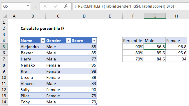
To calculate a conditional percentile, you can use an array formula using the IF function inside the PERCENTILE function. See example below:

Formula

=PERCENTILE(IF(criteria,values),k)

Note: This is an array formula and must be entered with control + shift + enter.

Explanation

In the example shown, the formula in G5 is:

=PERCENTILE(IF(Table[Gender]=G$4,Table[Score]),$F5)

Where “Table” is an Excel Table with data in B5:D14.

How this formula works

This formula sits inside a small summary table with percentile values in column F and gender values in G4 and H4.

Working from the inside out, the IF function is set up like this:

IF(Table[Gender]=G$4,Table[Score])

Here, each value in the gender column is tested against the value in G4, “Male”.

The result is an array of boolean values like this:

{88;85;77;FALSE;FALSE;FALSE;83;FALSE;FALSE;79}

Only scores associated with males make it into the array, female scores are translated to FALSE. This array goes into the PERCENTILE function with the k value from F5, 90%.

PERCENTILE automatically ignores FALSE values and returns a result of 86.8.

The reference to Gender in G$4 is locked to prevent the row from changing. The reference to k values, $F5 is locked to prevent the column from changing. As a result, the formula can be copied across the range G5:H7.