How To Create Loan Amortization Schedule in Excel
This example teaches you how to create a loan amortization schedule in Excel.
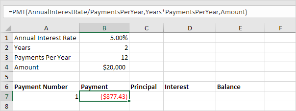
1. We use the PMT function to calculate the monthly payment on a loan with an annual interest rate of 5%, a 2-year duration and a present value (amount borrowed) of $20,000. We have named the input cells.
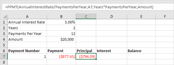
2. Use the PPMT function to calculate the principal part of the payment. The second argument specifies the payment number.
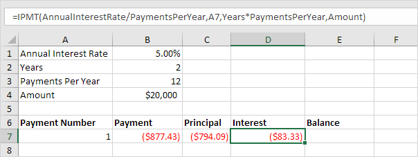
3. Use the IPMT function to calculate the interest part of the payment. The second argument specifies the payment number.
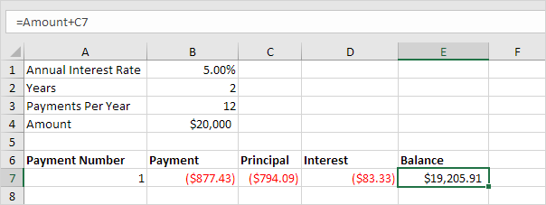
4. Update the balance.
5. Select the range A7:E7 (first payment) and drag it down one row. Change the balance formula.
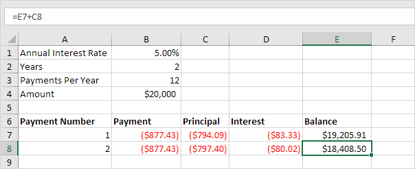
6. Select the range A8:E8 (second payment) and drag it down to row 30.
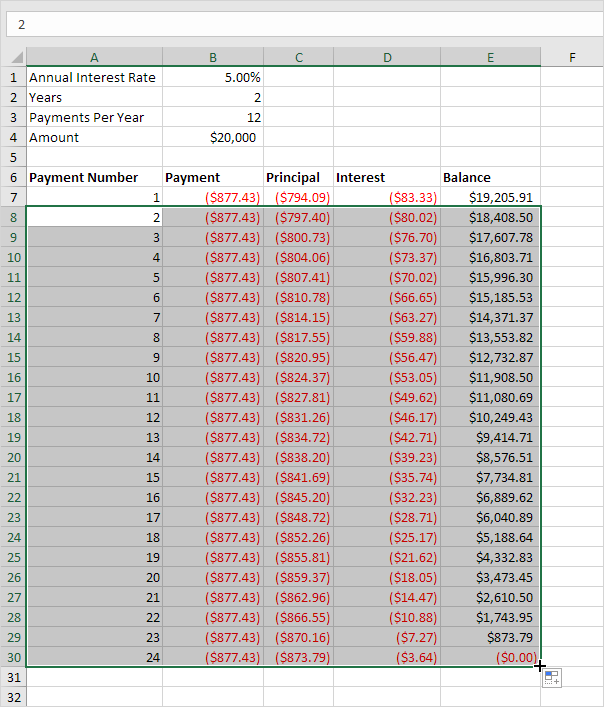
It takes 24 months to pay off this loan. See how the principal part increases and the interest part decreases with each payment.
