Calculate max or min change in a set of data in Excel

To calculate the max or min change in a set of data as shown, without using a helper column, you can use an array formula. See basic array formula example below:

Formula

{=MAX(range1-range2)}

Explanation

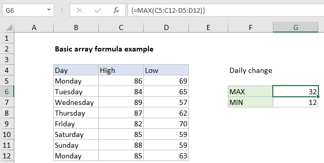
In the example, the formula in G6 is:

{=MAX(C5:C12-D5:D12)}

Note: this is an array formula and myst be entered with control + shift + enter.

How this formula works

The example on this page shows a simple array formula. Working from the inside out, the expression:

C5:C12-D5:D12

Results in an array containing seven values:

{17;19;32;25;12;26;29;22}

Each number in the array is the result of subtracting the “low” from the “high” in each of the seven rows of data. This array is returned to the MAX function:

=MAX({17;19;32;25;12;26;29;22})

And MAX returns the maximum value in the array, which is 32.

MIN change

To return the minimum change in the data, you can substitute the MIN function for the MAX function:

{=MIN(C5:C12-D5:D12)}

As before,  this is an array formula and myst be entered with control + shift + enter.