How to split text string at specific character in Excel

To split a text string at a certain character, you can use a combination of the LEFT, RIGHT, LEN, and FIND functions.

Formula

=LEFT(text,FIND(character,text)-1)

Explanation

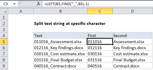
In the example shown, the formula in C5 is:

=LEFT(B5,FIND("_",B5)-1)

And the formula in D5 is:

=RIGHT(B5,LEN(B5)-FIND("_",B5))

How these formulas work

The first formula uses the FIND function to locate the underscore(_) in the text, then we subtract 1 to move back to the “character before the special character”.

FIND("_",B5)-1

In this example , FIND returns 7, so we end up with 6.

This result is fed into the LEFT function like as “num_chars” – the number of characters to extract from B5, starting from the left:

=LEFT(B5,6)

The result is the string “011016”.

To get the second part of the text, we use FIND with the right function.

We again use FIND to locate the underscore (7), then subtract this result from the total length of the text in B5 (22), calculated with the LEN function:

LEN(B5)-FIND("_",B5)

This gives us 15 (22-7), which is fed into the RIGHT function as “num_chars” –  – the number of characters to extract from B5, starting from the right:

=RIGHT(B5,15)