Split dimensions into three parts in Excel
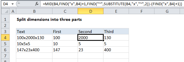
To split dimensions that like 100x50x25 into three separate parts, you can use some rather complicated formulas that use LEFT, MID, RIGHT, FIND, LEN, and SUBSTITUTE.
Note: you can also use Flash Fill in Excel 2013 and above, and the “text to columns” feature in older versions of Excel. Both approaches are quite a bit simpler than the formulas described below. However, if you need a dynamic solution, read on…
Formula
=LEFT(B4,FIND("x",B4)-1)

Explanation
The 1st dimension
To get the first dimension, we are using this formula in C4:
=LEFT(B4,FIND("x",B4)-1)
This works by extracting text starting at the LEFT. The number of characters is calculated by locating the first “x” in the text using the FIND function, then subtracting 1.
The 2nd dimension
To get the second dimension, we are using this formula in D4:
=MID(B4,FIND("x",B4)+1,FIND("~",SUBSTITUTE(B4,"x","~",2))-(FIND("x",B4)+1))
This formula uses the MID function, which extracts a certain number of characters starting at a certain position in the next. The starting position is calculated with this:
FIND("x",B4)+1
Which simply locates the first “x” and adds 1.
The number of characters is calculated using:
FIND("~",SUBSTITUTE(B4,"x","~",2))-(FIND("x",B4)+1)
We use SUBSTITUTE with FIND to locate the position of the 2nd “x”, as described here.
We then subtract from that the location of the first “x” + 1.
The 3rd dimension
To get the third dimension, we are using this formula in E4:
=RIGHT(B4,LEN(B4)-FIND("~",SUBSTITUTE(B4,"x","~",2)))
This uses the RIGHT function to extract a specific number of characters, starting from the right. We calculate the number of characters to extract by getting the total length with LEN, then subtracting the location of the 2nd instance of “x”.