
Split text and numbers in Excel
To separate text and numbers, you can use a formula based on the FIND function, the MIN function, and the LEN function with the LEFT or RIGHT function, depending on whether you want to extract the text or the number.
Formula
=MIN(FIND({0,1,2,3,4,5,6,7,8,9},A1&"0123456789"))
Explanation
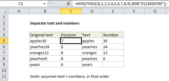
In the example shown, the formula in C5 is:
=MIN(FIND({0,1,2,3,4,5,6,7,8,9},B5&"0123456789"))
which returns 7, the position of the number 3 in the string “apples30”.
Overview
The formula looks complex, but the mechanics are in fact quite simple.
As with most formulas that split or extract text, the key is to locate the position of the thing you are looking for. Once you have the position, you can use other functions to extract what you need.
In this case, we are assuming that numbers and text are combined, and that the number appears after the text. From the original text, which appears in one cell, you want to split the text and numbers into separate cells, like this:
| Original | Text | Number |
| Apples30 | Apples | 30 |
| peaches24 | peaches | 24 |
| oranges12 | oranges | 12 |
| peaches0 | peaches | 0 |
As stated above, the key in this case is to locate the starting position of the number, which you can do with a formula like this:
=MIN(FIND({0,1,2,3,4,5,6,7,8,9},A1&"0123456789"))
Once you have the position, to extract just the text, use:
=LEFT(A1,position-1)
And, to extract just the number, use:
=RIGHT(A1,LEN(A1)-position+1)
How the formula works
In the first formula above, we are using the FIND function to locate the starting position of the number. For the find_text, we are using the array constant {0,1,2,3,4,5,6,7,8,9}, this causes the FIND function to perform a separate search for each value in the array constant. Since the array constant contains 10 numbers, the result will be an array with 10 values. For example, if original text is “apples30” the resulting array will be:
{8,10,11,7,13,14,15,16,17,18}
Each number in this array represents the position of an item in the array constant inside the original text.
Next the MIN function returns the smallest value in the list, which corresponds to the position in of the first number that appears in the original text. In essence, the FIND function gets all number positions, and MIN gives us the first number position: notice that 7 is the smallest value in the array, which corresponds to the position of the number 3 in original text.
You might be wondering about the odd construction for within_text in the find function:
B5&"0123456789"
This part of the formula concatenates every possible number 0-9 with the original text in B5. Unfortunately, FIND doesn’t return zero when a value isn’t found, so this is just a clever way to avoid errors that could occur when a number isn’t found.
In this example, since we are assuming that the number will always appear second in the original text, it works well because MIN forces only the smallest, or first occurrence, of a number to be returned. As long as a number does appear in the original text, that position will be returned.
If original text doesn’t contain any numbers, a “bogus” position equal to the length of the original text + 1 will be returned. With this bogus position, the LEFT formula above will still return the text and RIGHT formula will return an empty string.