Excel VLOOKUP and HLOOKUP functions Examples
Learn all about Excel’s lookup & reference functions such as the VLOOKUP, HLOOKUP, CHOOSE, MATCH and INDEX function.
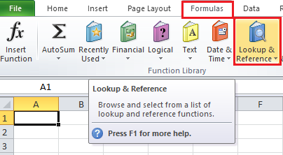
Navigation: Formula Tab → Function Library Group → Lookup and Reference
Vlookup
VLOOKUP stands for Vertical lookup. The VLOOKUP function looks for a value in the leftmost column of a table, and then returns a value in the same row from another column you specify.
Syntax for VLOOKUP function: VLOOKUP(lookup_value, table_array, col_index_num, [range_lookup])
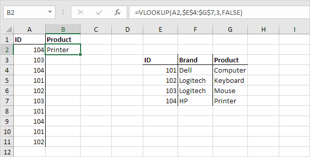
1. Insert the VLOOKUP function shown below.
Explanation
The VLOOKUP function looks for the ID (104) in the leftmost column of the range $E$4:$G$7 and returns the value in the same row from the third column (third argument is set to 3). The fourth argument is set to FALSE to return an exact match or a #N/A error if not found.
2. Drag the VLOOKUP function in cell B2 down to cell B11.
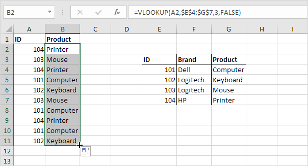
Note: when we drag the VLOOKUP function down, the absolute reference ($E$4:$G$7) stays the same, while the relative reference (A2) changes to A3, A4, A5, etc. Visit our page about the VLOOKUP function for much more information and many examples.
Hlookup
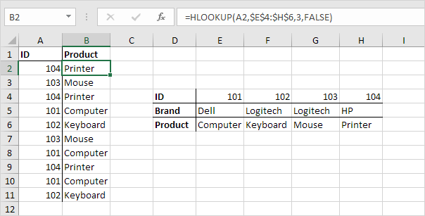
HLOOKUP stands for Horizontal lookup.
Syntax for HLOOKUP function : HLOOKUP(lookup_value, table_array, row_index_num, [range_lookup])
Choose
The CHOOSE function returns a value from a list of values, based on a position number.
Syntax for CHOOSE function: CHOOSE(index_num, value1, [value2], …)

Explanation: Boat found at position 3.
Match
The MATCH function returns the position of a value in a given range.
Syntax for MATCH function: MATCH(lookup_value, lookup_array, [match_type])
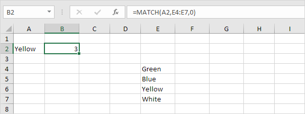
Explanation: Yellow found at position 3 in the range E4:E7. The third argument is optional. Set this argument to 0 to return the position of the value that is exactly equal to lookup_value (A2) or a #N/A error if not found. Use INDEX and MATCH and become an Excel pro.
Index
The INDEX function below returns a specific value in a two-dimensional range.
Syntax for INDEX function: INDEX(array, row_num, [column_num])
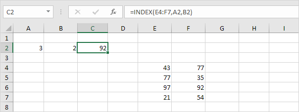
Explanation: 92 found at the intersection of row 3 and column 2 in the range E4:F7.
The INDEX function below returns a specific value in a one-dimensional range.
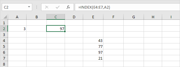
Explanation:
97 found at position 3 in the range E4:E7. .
