How to Use RANK function in Excel
The RANK function returns the rank of a number in a list of numbers. RANK gives duplicate numbers the same rank.
This tutorials shows how to rank a set of numeric values, where the highest value is ranked #1 in Excel.
To achieve this you can use the RANK function.
Formula
=RANK(value,data)
See Examples of Excel Rank function below:
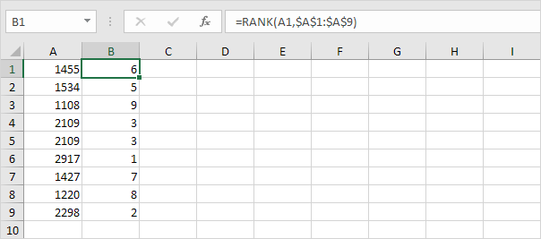
1. If the third argument is omitted (or 0), Excel ranks the largest number first, second largest number second, etc.

Note: when we drag the RANK function down, the absolute reference ($A$1:$A$9) stays the same, while the relative reference (A1) changes to A2, A3, A4, etc.
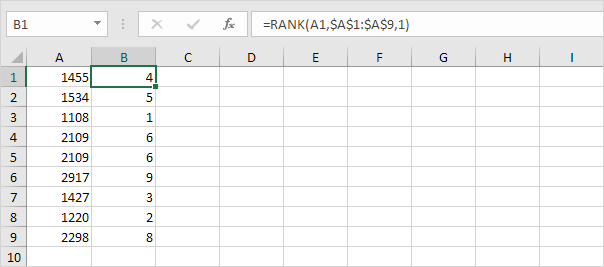
2. If the third argument is 1, Excel ranks the smallest number first, second smallest number second, etc.

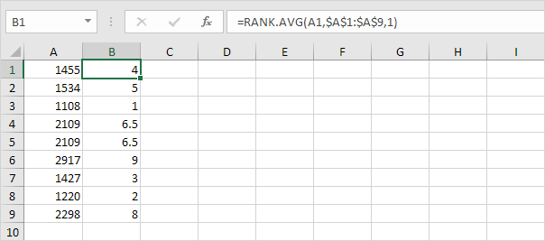
3. Use the RANK.AVG function to return the average rank if more than one number has the same rank.

4.

Explanation
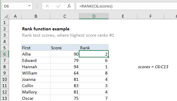
In the example shown, the formula in D6 is:
=RANK(C6,scores)
Where scores is the named range C6:C13.
How this formula works
You can use the RANK function to rank numeric values.
RANK has two modes of operation: ranking values where the largest value is #1 (order = 0), and ranking values where the lowest value is #1 (order = 1).
In this case, we are ranking test scores, so the highest value should rank #1, so we omit the order argument, which defaults to zero:
=RANK(C6,scores)
The following formula, which includes order set to zero, is equivalent:
=RANK(C6,scores,0)