Highlight numbers that include symbols in Excel

This tutorial shows how to Highlight numbers that include symbols in Excel using the example below;

Formula

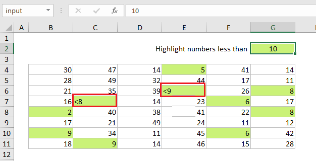
=IF(ISNUMBER(B4),B4<input,IF(LEFT(B4)="<",(MID(B4,2,LEN(B4))+0)<input))

Explanation

To highlight numbers less than a certain value, including numbers entered as text like “<9”, “<10”, etc., you can use conditional formatting with a formula strips the symbols as needed and handles the result as a number. In the example shown, “input” is a named range for cell G2.

How this formula works

The formula first uses the ISNUMBER function to test if the value is a number, and applies a simple logical if so:

=IF(ISNUMBER(B4)

For any number less than the value in “input”, the formula will return TRUE and the conditional formatting will be applied.

However, if the value is not a number, the formula then checks if the first character is a less than symbol (<) using the LEFT function:

IF(LEFT(B4)="<"

If so, the MID function is used to extract everything after the symbol:

MID(B4,2,LEN(B4)

Technically, the LEN function returns a number 1 greater than we need, since it includes the “<” symbol as well. If this bothers you, feel free to subtract 1.

The result of MID is always text so the formula adds zero to force a Excel to convert the text to a number. This number is then compared to the value from “input”.