Highlight rows with dates between In Excel
This tutorial shows how to Highlight rows with dates between In Excel using the example below;
Formula
=AND($A1>=start,$A1<=end)

Explanation
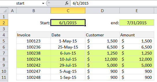
If you want to highlight rows that contain dates between two dates with conditional formatting, you can use a formula based on the AND and DATE functions. In the example, shown, the range B5:E11 has a conditional formatting rule applied using this formula:
=AND($C5>=start,$C5<=end)
Note: it’s important that CF formulas be entered relative to the “active cell” in the selection, which is assumed to be B5 in this case.
This formula refers to two named ranges: start (C2) and end (E2).
How this formula works
The AND function takes multiple arguments and returns TRUE only when all arguments return TRUE. Dates are just serial numbers in Excel, so earlier dates are always less than later dates. In the above formula, any dates that are greater than or equal to the start date AND less than or equal to the end date will pass both tests and the AND function will return TRUE, triggering the rule.
References to the start and end dates (C2 and E2) are absolute and will not change. References to the date in column C are “mixed” — the column is locked, but the row number is free to change.
Without named ranges
This formula refers to two named ranges: start (C2) and end (E2). Without using named ranges, the formula would look like this:
=AND($C5>=$C$2,$C5<=$E$2)
Embedding dates
This formula exposes the start and end input values directly on the worksheet, so that they can be easily changed. If you want to instead embed (hard-code) the dates directly into the formula, the formula would look like this:
=AND($C5>=DATE(2015,6,1),$C5<=DATE(2015,7,31))
The DATE function ensures that the date is properly recognized. It creates a proper Excel date with given year, month, and day values.