Highlight dates that are weekends in Excel

If you want to use conditional formatting to highlight dates occur on weekends (i.e. Saturday or Sunday),  you can use a simple formula based on the WEEKDAY function.

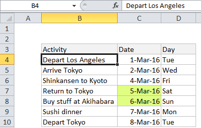
For example, if you have dates in the range C4:C10, and want to weekend dates, select the range C4:C10 and create a new conditional formatting rule that uses this formula:

=OR(WEEKDAY(C4)=7,WEEKDAY(C4)=1)

Note: it’s important that CF formulas be entered relative to the “active cell” in the selection, which is assumed to be C5 in this case.

Once you save the rule, you’ll see all dates that are a Saturday or a Sunday highlighted by your rule.

How this formula works

This formula uses the WEEKDAY function to test dates for either a Saturday or Sunday. When given a date, WEEKDAY returns a number 1-7, for each day of the week. In it’s standard configuration, Saturday = 7 and Sunday = 1. By using the OR function, use WEEKDAY to test for either 1 or 7. If either is true, the formula will return TRUE and trigger the conditional formatting.

Highlighting the entire row

If you want to highlight the entire row, apply the conditional formatting rule to all columns in the table and lock the date column:

=OR(WEEKDAY($C4)=7,WEEKDAY($C4)=1)