Highlight cells that contain in Excel

Note: Excel contains many built-in “presets” for highlighting values with conditional formatting, including a preset to highlight cells that contain specific text. However, if you want more flexibility, you can use your own formula, as explained in this article.

If you want to highlight cells that contain certain text, you can use a simple formula that returns TRUE when a cell contains the text (substring) that you specify.

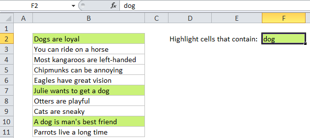
For example, if you want to highlight any cells in the range B2:B11 that contain the text “dog”, you can use:

=ISNUMBER(SEARCH("dog",B2))

Note: with conditional formatting, it’s important that the formula be entered relative to the “active cell” in the selection, which is assumed to be B2 in this case.

How this formula works

When you use a formula to apply conditional formatting, the formula is evaluated relative to the active cell in the selection at the time the rule is created. In this case, the rule is evaluated for each of the 10 cells in B2:B11, and B2 will change to the address of the cell being evaluated each time, since B2 is relative.

The formula itself uses the SEARCH function to find the position of “dog” in the text. If “dog” exists, SEARCH will return a number that represents the position. If “dog” doesn’t exist, SEARCH will return a #VALUE error. By wrapping ISNUMBER around SEARCH, we trap the error, so that the formula will only return TRUE when SEARCH returns a number. We don’t care about the actual position, we only care if there is a position.

Case sensitive option

SEARCH is not case-sensitive. If you need to check case as well, just replace SEARCH with FIND like so:

=ISNUMBER(FIND("dog",A1))