Conditional formatting based on another cell in Excel

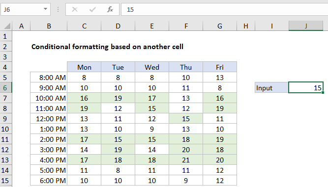
This tutorial shows how to Conditionally format based on another cell in Excel using the example below;

Formula

=A1>=$J$1

Explanation

To apply conditional formatting based on a value in another cell, you can create a rule based on a simple formula. In the example shown, the formula used to apply conditional formatting to the range C5:G15 is:

=C5>=$J$6

How this formula works

Excel contains many built-in “presets” for highlighting values with conditional formatting, including a preset to highlight cells greater than a specific value. However, by using your own formula, you have more flexibility and control.

In this example, a conditional formatting rule is set up to highlight cells in the range C5:G15 when then are greater than the value entered in cell J6. The formula used to create the rule is:

=C5>=$J$6

The rule is applied to the entire range C5:G15, and the value in J6 can be changed at any time by the user. When a new value is entered, the highlighting is immediately updated.

The formula uses the greater than or equal to operator (>=) to evaluate each cell in the range against the value in J6. The reference to C5 is relative and changes as the formula is evaluated for each cell in the range. The reference to cell J6 is “locked” as an absolute reference ($J$6).

When a value in the range is greater than or equal to 15 (the current value in J6), the formula returns TRUE and the rule is triggered.