Two-way lookup with INDEX and MATCH in Excel

This tutorial shows how to calculate Two-way lookup with INDEX and MATCH in Excel using the example below;

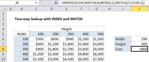
Formula

=INDEX(data,MATCH(val,rows,1),MATCH(val,columns,1))

To lookup in value in a table using both rows and columns, you can build a formula that does a two-way lookup with INDEX and MATCH.

In the example shown, the formula in J8 is:

=INDEX(C6:G10,MATCH(J6,B6:B10,1),MATCH(J7,C5:G5,1))

Note that this formula is doing and “approximate match”, so row values and column values must be sorted.

The core of this formula is INDEX, which is simply retrieving a value from C6:G10 (the “data”) based on a row number and a column number.

=INDEX(C6:G10, row, column)

To get the row and column numbers, we use MATCH, configured for approximate match, by setting the 3rd argument to 1 (TRUE):

MATCH(J6,B6:B10,1) // get row number
MATCH(J7,C5:G5,1) // get column number

In the example, MATCH will return 2 when width is 290, and 3 when height is 300.

In the end, the formula reduces to:

=INDEX(C6:G10, 2, 3)
= 1800