VLOOKUP by date in Excel
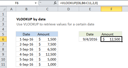
This tutorial shows how to calculate VLOOKUP by date in Excel using the example below;
Formula
=VLOOKUP(date,table,col,FALSE)

Explanation
To retrieve a value on a specific date from a table, you can use the VLOOKUP function.
In the example shown, the formula in F6 is:
=VLOOKUP(E6,B6:C11,2,0)
How this formula works
This is a standard VLOOKUP formula. It requires a table with lookup values (in this case, dates) to the left of the values being retrieved.
The lookup value comes from cell E6, which must be a valid date. The table array is the range B6:C11, and the column index is 2, since the amounts are in the second column of the table. Finally, zero is provided for the final argument to force an exact match.
The VLOOKUP function locates the date value for Sept 4, and returns the value at the same row in the second column: 12,500.
Note: the lookup value and the date values in the table must be valid Excel dates.