Multiple matches in comma separated list in Excel
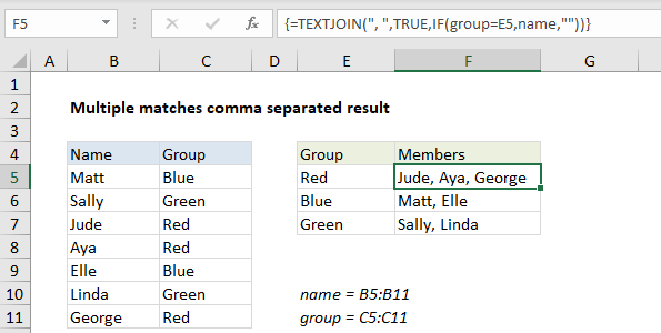
This tutorial shows how to work Multiple matches in comma separated list in Excel using the example below;
Formula
{=TEXTJOIN(", ",TRUE,IF(range1=E5,range2,""))}

Explanation
To lookup and retrieve multiple matches in a comma separated list (in a single cell) you can use the IF function with the TEXTJOIN function. In the example shown, the formula in F5 is:
{=TEXTJOIN(", ",TRUE,IF(group=E5,name,""))}
This is an array formula and must be entered with control + shift + enter.
This formula uses the named ranges “name” (B5:B11) and “group” (C5:C11).
How this formula works
The core of this formula is the IF function, which “filters” the names in the table by color like this:
IF(group=E5,name,""))
The logical test checks each cell in the named range “group” for the color value in E5 (red in this case). The result is an array like this:
{FALSE;FALSE;TRUE;TRUE;FALSE;FALSE;TRUE}
That result is used in turn to filter names from the named range “name”:
{"Matt";"Sally";"Jude";"Aya";"Elle";"Linda";"George"}
For each TRUE, the name survives, for each FALSE, IF returns an empty string (“”).
The result of IF looks is this array:
{"";"";"Jude";"Aya";"";"";"George"}
which goes into the TEXTJOIN function as text1.
TEXTJOIN is configured to use a comma as the delimiter, and to ignore empty values. The final result is this text string:
“Jude, Aya, George”
Multiple conditions
You can’t use the AND or OR functions in an array formula like this because they only return a single result. You can use boolean logic like this for AND:
=TEXTJOIN(", ",TRUE,IF((condition1)*(condition2),name,""))
Note: TEXTJOIN was introduced in Excel 2016 via Office 365.