Get cell content at given row and column in Excel

This tutorial shows how to Get cell content at given row and column in Excel using the example below;

Formula

=INDIRECT(ADDRESS(row,col))

Explanation

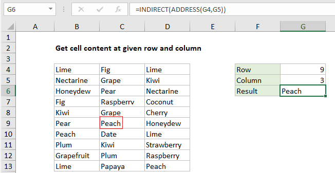
To get cell content with a given row and column number, you can use the ADDRESS function together with INDIRECT. In the example shown, the formula in G6 is:

=INDIRECT(ADDRESS(G4,G5))

How this formula works

The Excel ADDRESS function returns the address for a cell based on a given row and column number. For example, the ADDRESS function with 1 for both row and column like this:

=ADDRESS(1,1)

returns “$A$1” as text.

The INDIRECT function returns a valid reference from a text string.

In the example shown, the ADDRESS function returns the value “$C$9” inside INDIRECT:

=INDIRECT("$C$9")

The INDIRECT then this text into a normal reference and returns the value in cell C9, which is “Peach”.

Note: INDIRECT is a volatile function and can cause performance problems in more complicated worksheets.

With INDEX

By feeding the INDEX function an array that begins at A1, and includes cells to reference, you can get the same result with a formula that may be easier to understand. For example, the formula below will return the same result as seen in the screenshot.

=INDEX(A1:E100,G4,G5)

The size of the array is arbitrary, but it must to start at A1 and include the data you wish to reference.