Exact match lookup with INDEX and MATCH in Excel

{=INDEX(data,MATCH(TRUE,EXACT(val,lookup_col),0),col_num)}

Case-sensitive lookup

By default, standard lookups with VLOOKUP or INDEX + MATCH aren’t case-sensitive. Both VLOOKUP and MATCH will simply return the first match, ignoring case.

However, if you need to do a case-sensitive lookup, you can do so with an array formula that uses INDEX, MATCH, and the EXACT function.

In the example, we are using the following formula

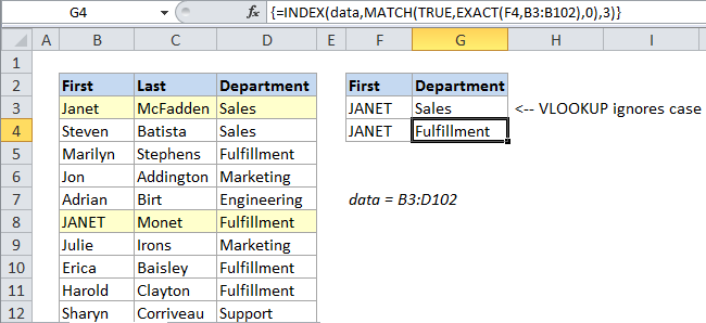
{=INDEX(data,MATCH(TRUE,EXACT(F4,B3:B102),0),3)}

This formula is an array formula and must be entered with Control + Shift + Enter.

How the formula works

Since MATCH alone isn’t case sensitive, we need a way to get Excel to compare case. The EXACT function is the perfect function for this, but the way we use it is a little unusual, because we need to compare one cell to a range of cells.

Working from the inside out, we have first:

EXACT(F4,B3:B102)

where F4 contains the lookup value, and B3:B102 is a reference to the lookup column (First names). Because we are giving EXACT an array as a second argument, we will get back an array of TRUE false values like this:

{FALSE,FALSE,FALSE,FALSE,FALSE,TRUE,etc.}

This is the result of comparing the value in B4 every cell in the lookup column. Wherever we see TRUE, we know we have an exact match that respects case.

Now we need to get the position (i.e. row number) of the TRUE value in this array. For this, we can use MATCH, looking for TRUE and set in exact match mode:

MATCH(TRUE,EXACT(F4,B3:B102),0)

It’s important to note that MATCH will always return the first match if there are duplicates, so if there happens to be another exact match in the column, you’ll only match the first one.

Now we have a row number. Next, we just need to use INDEX to retrieve the value at the right row and column intersection. The column number in this case is hard-coded as 3, since the named range data includes all columns. The final formula is:

{=INDEX(data,MATCH(TRUE,EXACT(F4,B3:B102),0),3)}

We have to enter this formula as an array formula because of the array created by EXACT.