Find longest string with criteria in Excel
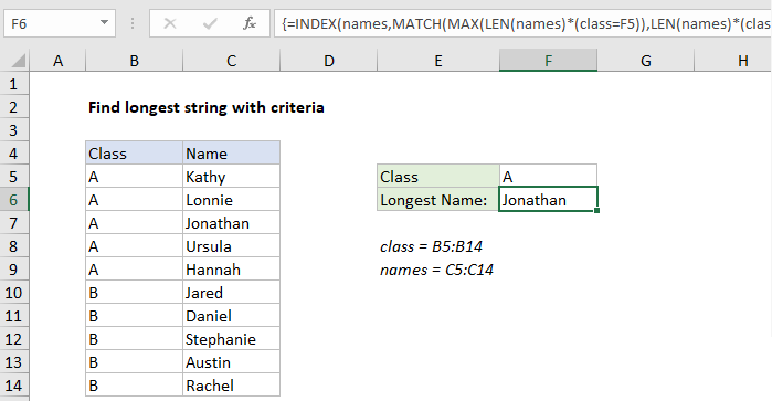
This tutorial shows how to Find longest string with criteria in Excel using the example below;
Formula
{=INDEX(range1,MATCH(MAX(LEN(range1)*(range2=criteria)),LEN(range1)*(range2=criteria),0))}

Explanation
To find the longest string in a range with criteria, you can use an array formula based on INDEX, MATCH, LEN and MAX. In the example shown, the formula in F6 is:
{=INDEX(names,MATCH(MAX(LEN(names)*(class=F5)),LEN(names)*(class=F5),0))}
Where “names” is the named range C5:C14, and “class” is the named range B5:B14.
Note: this is an array formula and must be entered with control + shift + enter.
How this formula works
The core of this formula is the MATCH function, which locates the position of the longest string using supplied criteria:
MATCH(MAX(LEN(names)*(class=F5)),LEN(names)*(class=F5),0)
Note MATCH is set up to perform an exact match by supplying zero for match type. For lookup value, we have:
LEN(names)*(class=F5)
The LEN function returns an array of results (lengths), one for each name in the list where class = “A” from cell F5 :
{5;6;8;6;6;0;0;0;0;0}
This effectively filters out all of Class B, and the MAX function then returns the largest value, 8.
To construct a lookup array, we use the same approach:
LEN(names)*(class=F5)
And get the same result:
{5;6;8;6;6;0;0;0;0;0}
After LEN and MAX run, we have a MATCH formula with these values:
MATCH(8,{5;6;8;6;6;0;0;0;0;0},0))
MATCH then returns the position of 8 in the list, 3, which feeds into INDEX like this:
=INDEX(names,3)
Finally, INDEX dutifully returns the value in the 3rd position of names, which is “Jonathan”.