Skip to content
Free Excel Tutorials
  • Home
  • Excel For Beginners
  • Excel Intermediate
  • Advanced Excel For Experts

Data Analysis

  • Chart Axes in Excel
  • Conditional Formatting Color Scales Examples in Excel
  • How To Insert and Customize Sparklines in Excel
  • How to Create Area Chart in Excel
  • Working With Tables in Excel

References

  • Approximate match with multiple criteria in Excel
  • Two-column Lookup in Excel
  • How to use Excel TRANSPOSE Function
  • Two-way lookup with VLOOKUP in Excel
  • How to get address of named range in Excel

Data Validations

  • Excel Data validation whole percentage only
  • Excel Data validation date in next 30 days
  • Excel Data validation exists in list
  • How To Create Drop-down List in Excel
  • Excel Data validation require unique number

Dynamic lookup table with INDIRECT in Excel

by

This tutorial shows how to calculate Dynamic lookup table with INDIRECT in Excel using the example below;

To allow a dynamic lookup table, you can use the INDIRECT function with named ranges inside of VLOOKUP.

Formula

=VLOOKUP(A1,INDIRECT("text"),column)

Explanation

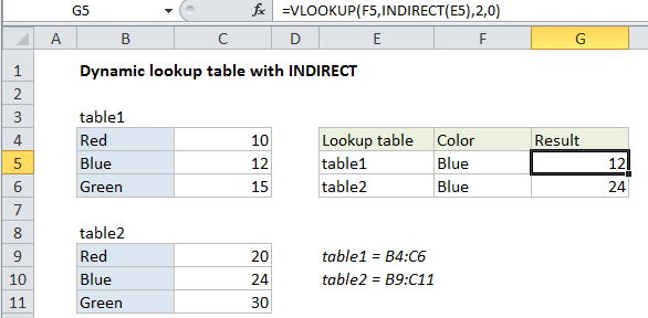
In the example shown the formula in G5 is:

=VLOOKUP(F5,INDIRECT(E5),2,0)

Background

The purpose of this formula is to allow an easy way to switch table ranges inside a lookup function. One way to handle is to create a named range for each table needed, then refer to the named range inside of VLOOKUP. However, if you just try to give VLOOKUP a table array in the form of text (i.e. “table1”) the formula will fail. The INDIRECT function is needed to resolve the text to a valid reference.

How this formula works

At the core, this is a standard VLOOKUP formula. The only difference is the use of INDIRECT to return a valid table array.

In the example shown, two named ranges have been created: “table1” refers to B4:C6, and “table2” refers to B9:C11*.

INDIRECT picks up the text in E5 (“table1”) and resolves it the named range table1, which resolves to B9:C11, which is returned to VLOOKUP.

VLOOKUP performs the lookup and returns 12 for the color “blue” in table1.

* Note: names ranges actually create absolute references like $B$9:$C$11, but I’ve omitted the absolute reference syntax to make the description easier to read.

Post navigation

Previous Post:

How to use Excel CHOOSE Function

Next Post:

Customize Ribbon In Excel

Leave a Reply Cancel reply

Your email address will not be published. Required fields are marked *

Learn Basic Excel

Ribbon
Workbook
Worksheets
Format Cells
Find & Select
Sort & Filter
Templates
Print
Share
Protect
Keyboard Shortcuts

Categories

  • Charts
  • Data Analysis
  • Data Validation
  • Excel Functions
    • Cube Functions
    • Database Functions
    • Date and Time Functions
    • Engineering Functions
    • Financial Functions
    • Information Functions
    • Logical Functions
    • Lookup and Reference Functions
    • Math and Trig Functions
    • Statistical Functions
    • Text Functions
    • Web Functions
  • Excel VBA
  • Excel Video Tutorials
  • Formatting
  • Grouping
  • Others

Logical Functions

  • How to use IFS function in Excel
  • Check multiple cells are equal in Excel
  • IF with boolean logic in Excel
  • IF function: Description, Usage, Syntax, Examples and Explanation
  • IFS function: Description, Usage, Syntax, Examples and Explanation

Date Time

  • WORKDAY.INTL function: Description, Usage, Syntax, Examples and Explanation
  • Get month from date in Excel
  • DAY function: Description, Usage, Syntax, Examples and Explanation
  • Get date from day number in Excel
  • How to calculate next scheduled event in Excel

Grouping

  • Map inputs to arbitrary values in Excel
  • Group times into unequal buckets in Excel
  • How to randomly assign data to groups in Excel
  • Group numbers with VLOOKUP in Excel
  • Calculate conditional mode with criteria in Excel

General

  • How to calculate percentage discount in Excel
  • How to Insert Cells, Row and Rows in Excel
  • Spell Check in Excel
  • Check if multiple cells have same value with case sensitive in Excel
  • Subtotal by invoice number in Excel
© 2026 xlsoffice . All Right Reserved. | Teal Smiles | Abbreviations And Their Meaning