nth largest value with criteria in Excel
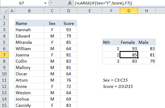
This tutorial shows how to calculate nth largest value with criteria in Excel using the example below;
To get the 2nd largest value, 3rd largest value, 4th largest value, and so on, where each value matches supplied criteria, you can use an array formula that uses the LARGE and IF functions.
Formula
{=LARGE(IF(range=criteria,values),n)}

Explanation
In the example shown, the formula in G7 is:
{=LARGE(IF(Sex="F",Score),F7)}
Where “Sex” is a named range for C3:C15 and “Score” is the named range D3:D15.
Note: this is an array formula and must be entered using Control + Shift + Enter.
How this formula works
The LARGE function is fully automatic — you just need to supply a range and an integer for”nth” to specify the ranked value you want.
The problem in this case is that we don’t want LARGE to operate on every value in the range, just values that are either male or female (M or F). To apply this criteria, we use the IF function, which provides a logical test for either “M” or ‘F”. Because we are applying the test to an array of values, the result will also be an array. In the example shown, the resulting array looks like this:
{93;FALSE;85;FALSE;81;FALSE;FALSE;FALSE;FALSE;72;FALSE;FALSE;83}
Where FALSE represents male scores (“F”) and numbers represent female scores.
The LARGE function will automatically ignore TRUE and FALSE values, so the result will be the nth largest value from the set of actual numbers in the array.