Minimum value if in Excel
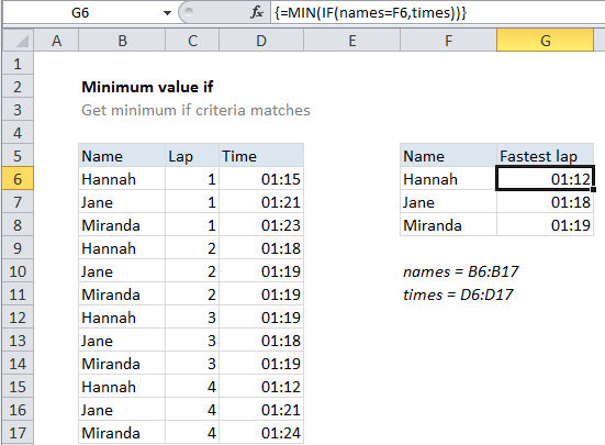
This tutorial shows how to calculate Minimum value if in Excel using the example below;
Formula
{=MIN(IF(range=criteria,values))}
Explanation
To get a minimum value based on criteria, you can use the MIN function together with the IF function. In the example shown, the formula in cell G6 is:
{=MIN(IF(names=F6,times))}
Where “names” is the named range B6:B17, and times is the named range D6:D17.
This is an array formula and must be entered with Control + Shift + Enter.
How this formula works
The IF function is evaluated first with the following logical test:
names=F6
This generates an array of TRUE / FALSE values, where TRUE corresponds to rows where the name matches the value in F6. The “value if true” for IF is the named range “times”, which returns the full set of times. The result is that the array from the logical test effectively “filters” the time values. When a result is TRUE, the time is passed into array returned by IF. When a result is FALSE, the time value is replaced by the boolean FALSE.
The MIN function then returns the minimum value in this array. FALSE values are automatically ignored.
With MINIFS
The MINIFS function, introduced in Excel 2016 via Office 365, is designed to calculate minimums based on one or more criteria without the need for an array formula. With MINIFS, the formula in G6 is:
=MINIFS(times,names,F6)