Max value ignore all errors in Excel

This tutorial shows how to calculate Max value ignore all errors in Excel using the example below;

Formula

=AGGREGATE(4,6,values)

Explanation

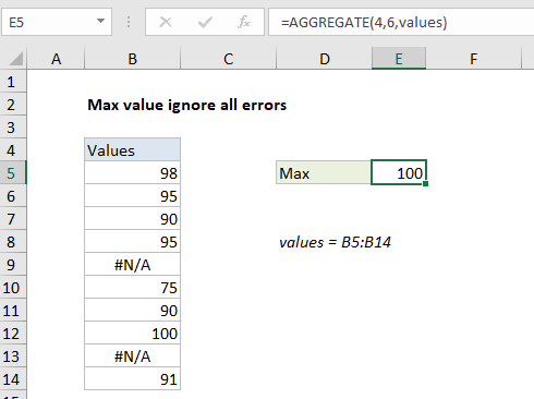
To get the maximum value in numeric data while ignoring all errors, you can use the AGGREGATE function, as explained below. In the example shown, the formula in E5 is:

=AGGREGATE(4,6,values)

where “values” is the named range B5:B14.

How this formula works

he AGGREGATE function can optionally ignore errors when calculating an a maximum value. To return the max value, while ignoring all errors in the data, you can use a formula like this:

=AGGREGATE(4,6,values)

Here, the number 4 specifies average, the number 6 is an option to ignore errors, and “values” is the named range B5:B14.

With these settings, AGGREGATE returns the maximum in the remaining eight values, 100.

Alternative with MAXIFS

The MAXIFS function can return the max value in a set of data, after applying one or more criteria to filter out unwanted values. If values in the data set are known to be positive, you can use the following formula to return the maximum value while ignoring errors:

=MAXIFS(values,values,">=0")

This works because the “greater or equal to zero” expression effectively filers out error values, and MAXIFS returns the maximum value from the remaining 8 values, 100.

Note: MAXIFS was introduced in Excel 2016 via Office 365.