Large with criteria in Excel
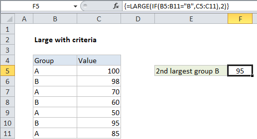
This tutorial shows how to calculate Large with criteria in Excel using the example below;
Formula
{=LARGE(IF(criteria,values),n)}

Explanation
To return the largest values in a set of data with criteria, you can use the a formula based on the LARGE and IF functions.
In the example shown, the formula in F5 is:
{=LARGE(IF(B5:B11="B",C5:C11),2)}
Note: this is an array formula and must be entered with control + shift + enter.
How this formula works
The LARGE function can be used to retrieve “nth” largest value in numeric data like so:
=LARGE(values,n)
In this example, we need include only values associated with group B. To do this, we use the IF function to filter:
IF(B5:B11="B",C5:C11)
Since we are running a logical test on an range of cells, we get an array of results:
{FALSE;98;FALSE;60;FALSE;95;FALSE}
Note that only values in group B make it into the array. Group A values become FALSE since they fail the logical test. This array is returned inside the LARGE function with 2 hardcoded as as “nth” (the argument “k” in LARGE):
=LARGE({FALSE;98;FALSE;60;FALSE;95;FALSE},2)
LARGE then returns 95, the second largest value in group B as the final result.
Multiple criteria
To take into account multiple criteria, you can extend the formula with boolean logic in a form like this:
=LARGE(IF((criteria1)*(criteria2),values),n)
Where criteria1 and criteria2 and represent an expression to test values in a criteria range, as shown in the original example above.