Sum by weekday in Excel

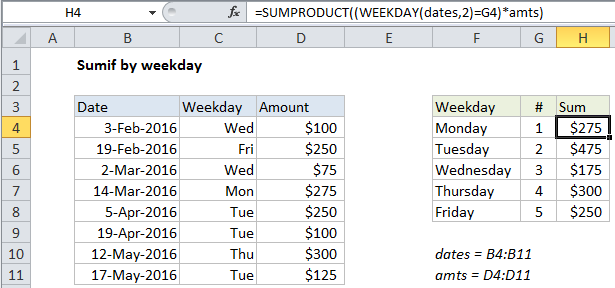
This tutorial shows how to Sum by weekday in Excel using the example below;

Formula

=SUMPRODUCT((WEEKDAY(dates)=day_num)*values)

Explanation

To sum data by weekday (i.e. sum by Mondays, Tuesdays, Wednesdays, etc.), you can use the SUMPRODUCT function together with the WEEKDAY function.

In the example shown, the formula in H4 is:

=SUMPRODUCT((WEEKDAY(dates,2)=G4)*amts)

How this formula works

You might wonder why we aren’t using the SUMIF or SUMIFS function? These appear to be an obvious way to sum by the days of the week. However, without adding a helper column with a weekday value, there is no way to create a criteria for SUMIF that takes into account the weekday.

Instead, we use the handy SUMPRODUCT function, which handles arrays gracefully without the need to use Control + Shift + Enter.

We are using SUMPRODUCT with just one argument, which consists of this expression:

(WEEKDAY(dates,2)=G4)*amts

Working from the inside out, the WEEKDAY function is configured with the optional argument 2, which causes it to return numbers 1-7 for the days Monday-Sunday, respectively. This is not necessary, but it makes it easier to list the days in order and pick up the numbers in column G in sequence.

WEEKDAY evaluates each value in the named range “dates” and returns a number. The result is an array like this:

{3;5;3;1;2;2;4;2}

The numbers returned by WEEKDAY are then compared to the value in G4, which is 1.

{3;5;3;1;2;2;4;2}=1

The result is an array of TRUE/FALSE values.

{FALSE;FALSE;FALSE;TRUE;FALSE;FALSE;FALSE;FALSE}

Next, this array is multiplied by the values in the named range “amts”.  SUMPRODUCT only works with numbers (not text or booleans) but math operations automatically coerce the TRUE/FALSE values to one’s and zeros, so we have:

{0;0;0;1;0;0;0;0}*{100;250;75;275;250;100;300;125}

Which yields:

{0;0;0;275;0;0;0;0}

With just this single array to process, SUMPRODUCT sums the items and returns the result.