Sum bottom n values with criteria in Excel

Explanation

To sum the bottom n values in a range matching criteria, you can use an array formula based on the SMALL function, wrapped inside the SUM function. In the generic form of the formula (above), range1 represents the range of cells compared to criteria, range2 contains numeric values from which bottom values are retrieved, and N represents “nth”.

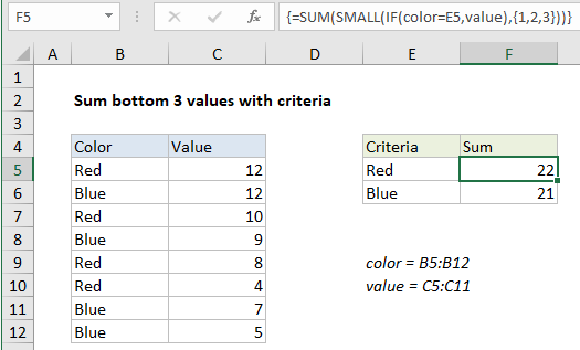
In the example, the active cell contains this formula:

=SUM(SMALL(IF(color=E5,value),{1,2,3}))

Where color is the named range B5:B12 and value is the named range C5:C12.

Note: this is an array formula and must be entered with control + shift + enter.

Here’s how the formula works

In its simplest form, SMALL returns the “Nth smallest” value in a range with this construction:

=SMALL (range,N)

So, for example:

=SMALL (C5:C12,2)

will return the 2nd smallest value in the range C5:C12, which is 5 in the example shown.

However, if you supply an “array constant” (e.g. a constant in the form {1,2,3}) to SMALL as the second argument, SMALL will return an array of results instead of a single result. So, the formula:

=SMALL (C5:C12, {1,2,3})

will return the 1st, 2nd, and 3rd smallest value C5:C12 in an array like this: {4,5,7}.

So, the trick here is to filter the values based on color before SMALL runs. We do this with an expression based on the IF function:

IF(color=E5,value)

This builds the array of values fed into SMALL. Essentially, only values associated with the color red make it into the array. Where color equals “red”, the array contains a number, and where the color is not red, the array contains FALSE:

SMALL({12;FALSE;10;FALSE;8;4;FALSE;FALSE},{1,2,3}))

The SMALL function ignores the FALSE values and returns the 3 smallest values in the array: {4,8,10}. The SUM function returns the final result, 22.