Two-way summary count with COUNTIFS in Excel

This tutorial shows how to work Two-way summary count with COUNTIFS in Excel using the example below;

Formula

=COUNTIFS(range1,critera1,range2,critera2)

Explanation

To build a two-way summary count (i.e. summarizing by rows and columns) you can use the COUNTIFS function.

In the example shown, the formula in G5 is:

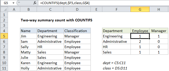
=COUNTIFS(dept,$F5,class,G$4)

How this formula works

The COUNTIFS function is designed to count things based on more than one criteria. In this case, the trick is to build a summary table first that contains one set of criteria in the left-most column, and a second set of criteria as column headings.

Then, inside COUNTIFS function, range1 is the named range “dept” (C5:C11) and the criteria comes from column F, input as the mixed reference $F5 (to lock the column). Range2 is the named range “class” (D5:D11) and the criteria comes from row 4, input as the mixed reference G$4 (to lock the row):

 =COUNTIFS(dept,$F5,class,G$4)

When this formula is copied through the table the mixed references change so that COUNTIFS will generate a count as the intersection of each “pair” of intersecting criteria.