Summary count with percentage breakdown in Excel

This tutorial shows Summary count with percentage breakdown in Excel using the example below;

Formula

=COUNTIF(range,criteria)/COUNTA(range)

Explanation

To generate a count with a percentage breakdown, you can use the COUNTIF or COUNTIFS function, together with COUNTA.

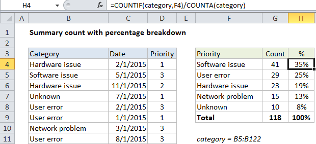
In the example shown the formula in H4 is:

=COUNTIF(category,F4)/COUNTA(category)

How this formula works

COUNTIF is set up to count cells in the named range “category”, which refers to B5:B122. The criteria is supplied as a reference to H4, which simply picks up the value in column F.

the COUNTA function simply counts all non-blank cells in the named range category (B5:B122) to generate a total count.

The COUNTIF result is divided by the COUNTA result to generate a percentage. All values in column H are formatted with the “Percentage” number format.

Note: since we already have a count per category in column G, it would be more efficient to pick the that count in this formula instead of recalculating the same count again in column H. However, COUNTIFS and COUNTA are shown together here for the sake of a complete solution.