Count unique numeric values with criteria in Excel

This tutorial shows how to Count unique numeric values with criteria in Excel using the example below;

Formula

{=SUM(--(FREQUENCY(IF(criteria,values),values)>0))}

Explanation

To count unique numeric values in a range with criteria you can use a formula based on the SUM and FREQUENCY functions, together with the IF function to apply criteria.

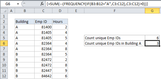
For example, assume you have a list of employee numbers with hours logged in two different buildings: building A, and building B. You want know how many unique employees logged time in each building. Since the same employee numbers appear more than once in the list, you need a formula that will count unique Employee IDs per building. In the example shown, the formula in G6 is:

{=SUM(--(FREQUENCY(IF(B3:B12="A",C3:C12),C3:C12)>0))}

Note: this is an array formula and must be entered with Control Shift Enter (CSE) syntax

How this formula works

The FREQUENCY function returns an array of values that correspond to “bins”. In this case, we are supplying a “filtered” set of ids for the data array, and the full set of ids for the bins array. The filtering is done with the IF function here:

IF(B3:B12="A",C3:C12)

Which in the example returns this:

{81400;81405;81405;82364;82364;FALSE;FALSE;FALSE;FALSE;FALSE}

Notice all ids not in building A are FALSE. Next, FREQUENCY returns an array of values that represent a count for each numeric value in the data array. This works because FREQUENCY has a special feature that automatically returns zero for numbers that appear more than once in the data array. The resulting array looks like this:

{1;2;0;2;0;0;0;0;0;0;0}

Next, each of these values is tested to be greater than zero. The result looks like this:

{TRUE;TRUE;FALSE;TRUE;FALSE;FALSE;FALSE;FALSE;FALSE;FALSE;FALSE}

Each TRUE in the list represents a unique number in the list, and we just need to add up the TRUE values with SUM. However, SUM won’t add up logical values in an array, so we need to first coerce the values into 1 or zero. This is done with the double-negative (–). The result an array of only 1’s or 0’s.

{1;1;0;1;0;0;0;0;0;0;0}

Finally, SUM adds these values up and returns the total, which in this case is 3.

Multiple criteria

You can extend the formula to handle multiple criteria like this:

{=SUM(--(FREQUENCY(IF((criteria1)*(criteria2),values),values)>0))}