Count cells that contain specific text in Excel

This tutorial shows how to Count cells that contain specific text in Excel using the example below;

Formula

=COUNTIF(range,”*text*”)

Explanation

To count the number of cells that contain certain text, you can use the COUNTIF function. In the example above “*” is a wildcard matching any number of characters.

In the example, the active cell contains this formula:

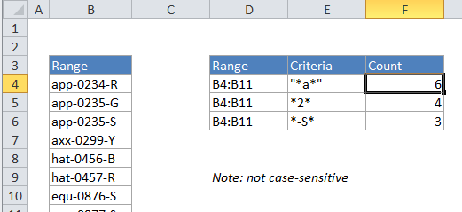
=COUNTIF(B4:B11,"*a*")

How this formula works

COUNTIF counts the number of cells in the range that contain “a” by matching the content of each cell against the pattern “*a*”, which is supplied as the criteria. The “*” symbol (the asterisk) is a wildcard in Excel that means “match any number of characters”, so this pattern will count any cell that contains “a” in any position. The count of cells that match this pattern is returned as a number.

You can easily adjust this formula to use the contents of another cell for the criteria. For example, if A1 contains the text you want to match, use the formula:

=COUNTIF(range,"*"&a1&"*")

Case-sensitive version

If you need a case-sensitive version, you can’t use COUNTIF. Instead you can test each cell in the range using a formula based on the FIND function and the ISNUMBER function, as explained here.

FIND is case-sensitive, and you’ll need to give it the range of cells and then use SUMPRODUCT to count the results. The formula looks like this:

=SUMPRODUCT(--(ISNUMBER(FIND(text,range))))

Note: FIND will return a number if text is found anywhere in the cell.