Count cells equal to one of many things

This tutorial shows how to Count cells equal to one of many things using the example below;

Formula

=SUMPRODUCT(COUNTIF(range,things))

Explanation

To count the number of cells equal to one of many values, you can use the COUNTIF function inside of SUMPRODUCT.

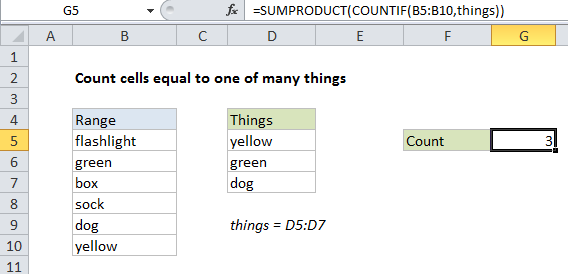
In the example shown, cell G5 contains this formula:

=SUMPRODUCT(COUNTIF(B5:B10,things))

Note COUNTIF is not case-sensitive.

How this formula works

COUNTIF counts the number of cells in the range that meet the criteria you supply. When you give COUNTIF a range of cells as the criteria, it returns an array of numbers as the result, where each number represents the count of one thing in the range. In this case, the named range “things” (D5:D7) contains 3 values, so COUNTIF returns 3 results in an array like:

=SUMPRODUCT({1;1;1})

since the values “yellow”, “green”, and “dog” all appear once in the range B5:B10. To handle this array, we use the SUMPRODUCT function, which is designed to work with arrays. SUMPRODUCT simply sums up the items in the array and returns the result, 3.

With array constant

With a limited number of values, you can use an array constant in your formula with SUM, like this:

=SUM(COUNTIF(B5:B10,{"red","green","blue"}))

But if you use cell references in the criteria. you’ll need to enter as an array formula or switch to SUMPRODUCT.