How To Use MaxIfs and MinIfs in Excel

This function combines the MAX and IF function in order to get the maximum value in a data set of Excel worksheet.

To look up the maximum value in a range based on specific criteria, you can use a basic array formula based on the IF function.

{=MAX(IF(criteria_range=criteria,value_range))}

Use the MAXIFS and MINIFS function in Excel 2016 to find the maximum and minimum value based on one criteria or multiple criteria.

1. For example, the MAXIFS function below finds the highest female score.

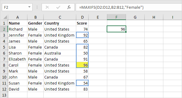
Note: the first argument (D2:D12 in this example) is always the range in which the maximum or minimum will be determined. This MAXIFS function has 1 range/criteria pair (B2:B12/Female).

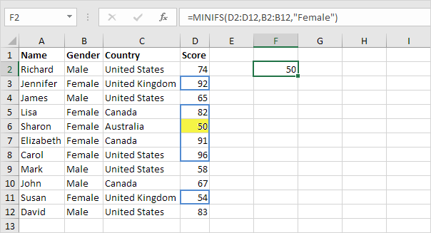
2. The MINIFS function below finds the lowest female score.

3. For example, the MAXIFS function below finds the highest female score in Canada.

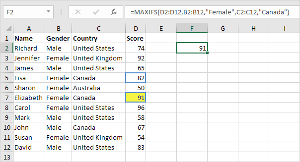
Note: this MAXIFS function has 2 range/criteria pairs (B2:B12/Female and C2:C12/Canada). The MAXIFS and MINIFS function can handle up to 126 range/criteria pairs.

4. The MAXIFS function below finds the highest score below 60.

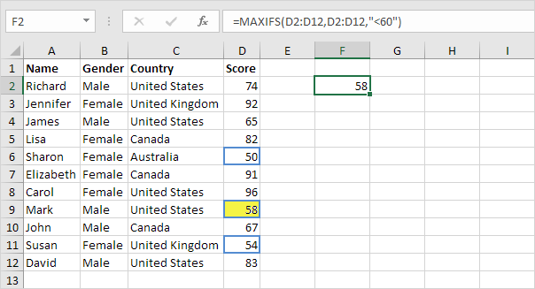
Note: this MAXIFS function only uses the range D2:D12.