How to use Excel INDEX Function

This Excel tutorial explains how to use the INDEX function with syntax and examples.

Excel INDEX Function Description

The Microsoft Excel INDEX function returns a value in a table based on the intersection of a row and column position within that table. The first row in the table is row 1 and the first column in the table is column 1.

The INDEX function is a built-in function in Excel that is categorized as a Lookup/Reference Function. The INDEX function can be entered as part of a formula in a cell of a worksheet.

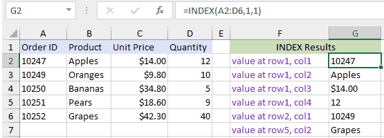
Explanation: Based on the example above, the INDEX would return:

=INDEX(A2:D6,1,1)
Result: 10247     'Intersection of row1 and col1 (cell A2)

=INDEX(A2:D6,1,2)
Result: "Apples"  'Intersection of row1 and col2 (cell B2)

=INDEX(A2:D6,1,3)
Result: $14.00    'Intersection of row1 and col3 (cell C2)

=INDEX(A2:D6,1,4)
Result: 12        'Intersection of row1 and col4 (cell D2)

=INDEX(A2:D6,2,1)
Result: 10249     'Intersection of row2 and col1 (cell A3)

=INDEX(A2:D6,5,2)
Result: Grapes    'Intersection of row5 and col2 (cell B6)

Return

The value at a given location.

Syntax

INDEX (array, row_num, [col_num], [area_num])

Arguments

array – A range of cells, or an array constant.
row_num – The row position in the reference or array.
col_num – [optional] The column position in the reference or array.
area_num – [optional] The range in reference that should be used.